


Afterword: Research Objectives and Significance
Viewed from a broader perspective, this study is not only concerned with proposing an alternative architecture for text generation, but also with clarifying a more general picture of learning in which representation, objective, and environment must be understood jointly. From this perspective, the three themes of this work are closely connected rather than independent. The first concerns how text should be represented and generated. The second concerns what kinds of objectives and evaluation criteria are genuinely aligned with such representations. The third concerns the kind of environment in which a model should ultimately learn if the goal is more general multimodal intelligence.
A useful starting point is to formalize learning itself as a model–environment interaction system. Let the environment be
\[ \mathcal{E} = (\Omega,\, \mathcal{O},\, \mathcal{A},\, \mathcal{T},\, \mathcal{F},\, \mathcal{G}), \tag{1} \]where \(\Omega\) is the environment state space, \(\mathcal{O}\) is the observation space, \(\mathcal{A}\) is the action or output space, \(\mathcal{T}\) is the state transition mechanism, \(\mathcal{F}\) is the feedback generation mechanism, and \(\mathcal{G}\) is the rule that converts feedback into optimization signals. Importantly, the notion of environment is understood here in a broad sense: it includes not only the external world, but also the data distribution presented to the model, task formats, supervision protocols, and even the loss rules by which feedback is transformed into gradients.
Let the model be denoted by \(M_\theta\), with internal state space \(\mathcal{H}\), state update map \(U_\theta\), and policy or generation map \(\Pi_\theta\). At interaction step \(t\), the closed-loop system can be written as
\[ \begin{aligned} o_t &\sim P_{\mathcal{E}}(\cdot \mid \omega_t), \\ h_t &= U_\theta(h_{t-1}, o_t), \\ a_t &\sim \Pi_\theta(\cdot \mid h_t), \\ \xi_t &\sim \mathcal{F}(\cdot \mid \omega_t, o_t, a_t), \\ \omega_{t+1} &\sim \mathcal{T}(\cdot \mid \omega_t, o_t, a_t, \xi_t), \\ \ell_t &= \mathcal{G}(\omega_t, o_t, a_t, \xi_t). \end{aligned} \]The overall learning objective is therefore
\[ \mathcal{J}(\theta;\, \mathcal{E}) \;=\; \mathbb{E}_{\tau \sim P(\tau \mid \theta, \mathcal{E})} \!\left[\sum_{t=1}^{T} \gamma^{t-1}\, \ell_t \right], \tag{2} \]where \(\tau\) denotes a complete interaction trajectory and \(\gamma\) is the discount factor.
This formalization shows directly that learning is never an isolated question of model structure alone. Rather, it is jointly determined by three factors: first, the state space in which the model absorbs and organizes information; second, the kind of feedback through which the environment defines improvement; and third, the actual structure that generates observations, transitions, and feedback. In this work, these three aspects correspond precisely to the three recurring themes of the paper: how text should be represented, which metrics are aligned with the true learning objective, and what kind of environment unified models are ultimately meant to enter.
1 · Rethinking text modeling: from state space to hierarchical generation
From a system-level perspective, the central question of text modeling is not merely which generation order to adopt, but rather in what kind of state text should be represented within the learning system. Mainstream autoregressive language models bind the state tightly to the surface token prefix, and generation is therefore written as
\[ p_{\mathrm{AR}}(x) = \prod_{t=1}^{n} p_\theta(x_t \mid x_{<t}). \tag{3} \]This factorization is highly effective, but it fundamentally corresponds to a strong modeling assumption: both global semantics and local realization are propagated through the same token-level conditional chain. In other words, it assumes that the surface string itself is the most natural and primary state space.
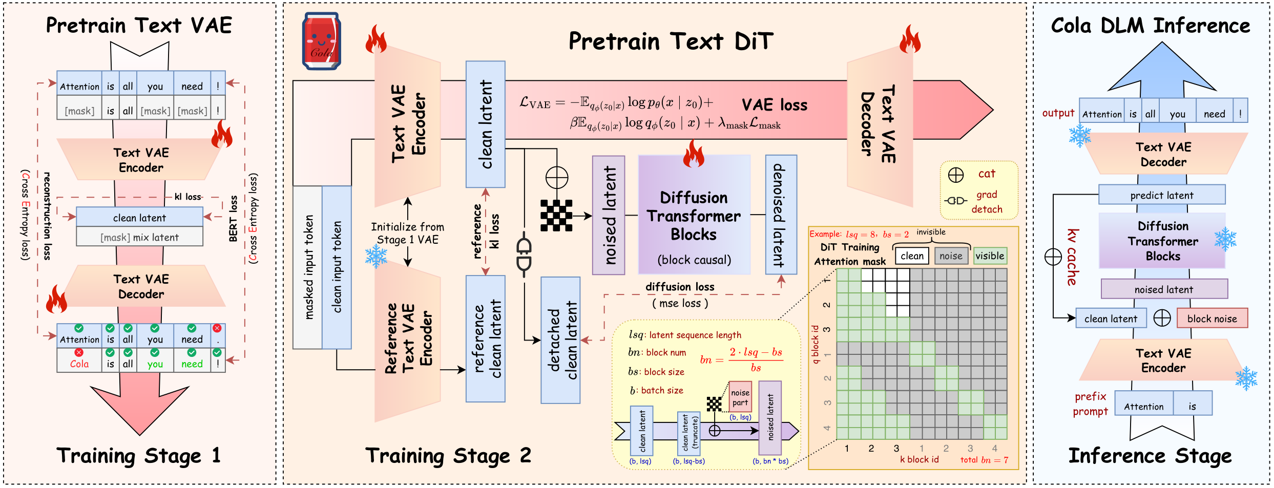
The route explored in this paper instead reconsiders text generation from the level of the state space itself. If text indeed contains a low-dimensional yet sufficiently useful global semantic structure, then a more natural approach is not to place the entire burden of generation on a token-level chain factorization, but to introduce latent variables explicitly and model high-level semantic organization separately from local textual realization. Correspondingly, the core factorization of Cola DLM is
\[ p(x, z_0) = p_\theta(x \mid z_0)\, p_\psi(z_0), \qquad p(x) = \int p_\theta(x \mid z_0)\, p_\psi(z_0)\, dz_0, \tag{4} \]where \(z_0\) is a continuous latent variable, \(p_\psi(z_0)\) is the latent prior, and \(p_\theta(x \mid z_0)\) is the conditional decoder. The crucial change here is not merely the introduction of latent variables, but the redefinition of the role of state in the system: the path no longer acts directly on observation recovery, but instead organizes global semantics in latent space first, after which the decoder carries out local textual realization.
This point can be stated compactly through the information decomposition of the average ELBO. Let \(q(x, z_0) := p_{\mathrm{data}}(x)\, q_\phi(z_0 \mid x)\); then
\[ \mathbb{E}_{p_{\mathrm{data}}(x)}\!\big[\mathcal{L}_{\mathrm{ELBO}}(x)\big] = \mathbb{E}_{q(x, z_0)}\!\big[\log p_\theta(x \mid z_0)\big] \,-\, I_q(X;\, Z_0) \,-\, \mathrm{KL}\!\big(\bar q_\phi(z_0)\,\|\,p_\psi(z_0)\big), \tag{5} \]where \(\bar q_\phi(z_0)\) is the aggregated posterior. This decomposition shows that hierarchical latent-space modeling breaks the text problem into three coupled but analytically distinguishable components: conditional realization, information compression, and prior matching. The latent variable is therefore not merely a continuous surrogate for discrete tokens, but an explicit intermediate state through which global semantic organization can be separated from local textual realization and modeled on its own terms.
From this perspective, compression must also be reconsidered. Prior work has emphasized the connection between compression and intelligence (Huang et al., 2024), while recent explorations of generation closer to raw data forms in images and videos, such as pixel-space modeling (Deng et al., 2026), further suggest that compression should not be equated with harmful information deletion. The key question is not whether every local detail is preserved, but whether the model can extract and organize structural information that is genuinely effective and generalizable. If text indeed admits a hierarchical structure in which high-level semantics and low-level realization are relatively separable, then reinterpreting text generation through informational hierarchy is not merely a change of method, but a theoretical re-evaluation of text modeling itself.
Accordingly, the first theme of this paper is not to reject autoregression, but to point out that autoregression occupies only one self-consistent, rather than unique, corner of the design space. If the data truly contains a hierarchy between low-dimensional global semantics and high-dimensional local realization, then organizing semantics first in a latent state and realizing text through conditional decoding may be closer to the true generative mechanism. Text generation should therefore not be understood solely as next-token fitting over discrete strings, but more generally as a systematic problem of how information is represented, compressed, and organized hierarchically.
2 · Continuous extension of discrete text: a shift in evaluation emphasis
Once the state space of the system is changed, the issue at the objective level changes accordingly. For conventional autoregressive language models, the training objective and evaluation quantities are naturally well aligned: maximum likelihood training directly corresponds to probability fitting over text, and likelihood and perplexity therefore have a clear and stable interpretation. In hierarchical continuous latent-space models, however, the actual training path is no longer direct token-level maximum likelihood, but a hierarchical objective jointly composed of reconstruction, latent prior learning, and representation regularization.
This can be seen from the relation between the ELBO and the true marginal likelihood:
\[ -\mathcal{L}_{\mathrm{ELBO}}(x) \;=\; -\log p_{\theta,\psi}(x) \;+\; \mathrm{KL}\!\big(q_\phi(z_0 \mid x)\,\|\,p_{\theta,\psi}(z_0 \mid x)\big). \tag{6} \]This shows that even at the level of the ELBO, the training objective is already separated from the true log-likelihood by a variational inference gap. Furthermore, in the actual training of Cola DLM, the model must jointly learn latent reconstruction, continuous prior fitting, and representation stabilization. The quantity being optimized is therefore not a single token-level likelihood in the classical sense.
For this reason, the mismatch should not be interpreted as a failure to learn, but rather as evidence that the model is learning something different. For autoregressive models and other paradigms that directly fit discrete distributions, likelihood and perplexity remain highly informative because they are naturally aligned with the training objective. For hierarchical continuous latent-space models, by contrast, the central issue is no longer whether local discrete distributions are fitted as sharply as possible, but whether higher-level semantic structures are effectively organized, whether the latent prior is well learned, and whether the final generations satisfy the actual task requirements.
From the perspective of systematic modeling, this phenomenon is in fact expected: when the state space expands from surface tokens to hierarchical latent variables, the optimization target correspondingly shifts from precise fitting of local discrete distributions to the organization of higher-level semantic structure, stable latent prior learning, and satisfaction of the true generative objective. For this route, generation-oriented metrics are therefore often more closely aligned with what the model is actually trained to do than perplexity. More importantly, model potential is often reflected more clearly in scaling behavior than in any single static likelihood value: what matters is whether capability continues to improve steadily as model size, data, and compute increase, rather than whether local fit under a particular pointwise metric is better.
This can also be connected to the perspective of the three governing curves developed in the theoretical analysis of the paper. For Cola DLM, the applicability of this route is not determined by a single likelihood value, but by whether three conditions hold simultaneously: the representation rate–distortion curve is already favorable at relatively low rate, the approximation error of the latent prior continues to decrease, and the inference gap remains controllable. In other words, the advantage of this route is not guaranteed automatically by latent variables or flow-based modeling themselves; it depends on whether the data truly contains a compressible global semantic structure, and whether the model can learn, fit, and realize that structure in a stable manner.
The second theme of this paper is therefore not merely that perplexity is inadequate, but that evaluation language itself must change once representation and objective have changed. For this class of models, generation quality and scaling behavior are often closer to the model's true capability and long-term potential than traditional perplexity.
3 · Unified models, model–environment interaction, and the value of multimodal unification
If we return again to the model–environment formalization in Eq. (1) and Eq. (2), the third theme becomes more natural. The importance of unified models does not lie merely in placing multiple modalities within a single parameterized network, but in changing the structure of the environment in which the model learns. In the real world, observations, transitions, and feedback are usually not generated independently across modalities; rather, they are often jointly determined by a shared latent state. A more general learning system therefore requires not a set of isolated modality interfaces placed side by side, but unified representations that can enter the same interaction state and share the same dynamical constraints.
This is closely related to two broader views of intelligence. One influential view understands intelligence as a collection of skills across tasks (Chollet, 2019). Under this view, a system becomes more capable because it can solve problems across more domains and under more diverse forms of supervision and interaction. The recent development of large language models partly reflects this tendency. A representative example is the progress of code agents that can operate within command-line environments. In such environments, the observation space, action space, and feedback mechanism are unusually well aligned with discrete symbolic representations. Interaction trajectories are easy to record, and correctness is often straightforward to verify, so these environments provide dense and precise learning signals.
Another view, closer to the world-model perspective, holds that intelligence consists in acquiring an internal model of the structure and dynamics of the world. Recent work on world models (Tu et al., 2025) moves in this direction by seeking to learn richer environmental dynamics, thereby supporting stronger generalization and more realistic interaction. From this perspective, the question is not only how many tasks a model can solve, but whether it learns in an environment whose structure is rich enough to induce the right abstractions. The environment therefore becomes central: a model can only internalize the regularities that are actually present in the observations, transitions, and feedback it encounters.
This can also be written more formally. Let the observation at step \(t\) be multimodal,
\[ o_t = \big(o_t^{(1)},\, o_t^{(2)},\, \dots,\, o_t^{(M)}\big), \qquad o_t^{(m)} \in \mathcal{O}^{(m)}, \tag{7} \]and suppose there exists a joint latent state
\[ z_t = \Phi\!\left(o_t^{(1)},\, \dots,\, o_t^{(M)}\right), \tag{8} \]such that feedback and transition depend primarily on this joint state rather than on marginal factorizations over modalities:
\[ \xi_t,\, \omega_{t+1} \;\sim\; p\!\left(\xi_t,\, \omega_{t+1} \mid z_t,\, a_t\right). \tag{9} \]If the true environmental dynamics satisfy
\[ p\!\left(\xi_t,\, \omega_{t+1} \mid o_t,\, a_t\right) \;\neq\; \prod_{m=1}^{M} p_m\!\left(\xi_t^{(m)},\, \omega_{t+1}^{(m)} \mid o_t^{(m)},\, a_t^{(m)}\right), \tag{10} \]then the learning problem is structurally non-separable across modalities. In such a case, treating each modality as an independent channel and only combining them superficially is generally insufficient. The theoretical significance of unified models lies precisely in the fact that the environment itself is non-separable in the sense of Eq. (10): the regularities that determine useful feedback are joint regularities rather than regularities defined on the marginal distribution of each modality.
This clarifies why multimodal unification is not merely an engineering convenience. Its purpose is not simply to process multiple data types with one backbone, but to allow the model to learn in an environment whose observation, transition, and supervision structure more faithfully reflects the coupled regularities of the real world. In such an environment, both inputs and outputs may be multimodal; useful feedback may depend on how different modalities constrain each other jointly; and the learned internal state should ideally reflect these joint constraints.
This also explains why text has long been the most difficult component in unified models. Images and videos naturally operate in continuous spaces, whereas text is a prototypically discrete modality. If they are to enter a common interaction state and share latent dynamics, a severe representational mismatch immediately arises. This is precisely one of the central obstacles repeatedly identified in recent unified-model research (Deng et al., 2025). In this sense, the significance of Cola DLM lies not only in proposing another text generator, but in providing a natural interface through which discrete text can enter a continuous latent space.
If discrete text is mapped into a continuous latent variable through
\[ z^{\mathrm{text}} \sim q_\phi(z \mid x^{\mathrm{text}}), \qquad x^{\mathrm{text}} \sim p_\eta(x \mid z^{\mathrm{text}}), \tag{11} \]then text acquires an interface compatible with other continuous modalities. One may then define a unified interaction state
\[ \tilde z_t \;=\; \Psi\!\left(z_t^{\mathrm{text}},\, z_t^{\mathrm{img}},\, z_t^{\mathrm{vid}},\, \dots \right), \tag{12} \]and perform state evolution, decision making, and feedback modeling at this level. Equations (11)–(12) formalize why Cola DLM may matter beyond text generation itself: its role is not only to generate text through a different path, but to provide a bridge through which an intrinsically discrete modality can participate in a continuous multimodal interaction state. In other words, it reduces the structural mismatch that otherwise prevents text from naturally entering a shared continuous environment.
This is why the broader significance of Cola DLM is better understood through model–environment interaction than through single-modality benchmarks alone. If learning is viewed as the optimization of Eq. (2) in richer and more realistic environments, then unified models matter because they expand the environments in which the model can learn. If text is to participate fully in such environments, then a bridge such as that in Eq. (11) becomes especially desirable. In this sense, Cola DLM is not merely an alternative text generator; it can also be understood as a candidate mechanism for aligning discrete text with continuous multimodal learning systems.
4 · The three themes under a unified perspective
In summary, the three themes of this paper are not separate supplementary discussions, but three manifestations of the same systematic problem. The first concerns the representation level: whether text should be modeled entirely on the token surface, or whether higher-level semantics can be organized in an independent latent state. The second concerns the objective level: once the model is trained through latent transport, reconstruction, and regularization rather than direct token-level maximum likelihood, which metrics remain genuinely aligned with the learning problem. The third concerns the environment level: if learning is ultimately model–environment interaction, then what kind of environment future models should inhabit, and what representational interfaces are needed for different modalities to become compatible within it.
From this perspective, autoregressive language modeling occupies a self-consistent corner of the design space: representation is tightly bound to surface tokens, the training objective is direct likelihood maximization, and the environment is largely symbolic and text-centered. The route explored in this work changes all three assumptions simultaneously. It introduces a hierarchical latent-variable representation for text, thereby changing the representational assumption; it moves optimization away from direct token-level likelihood, thereby weakening the central interpretive role of perplexity; and it provides a continuous interface for discrete text, thereby making text potentially more compatible with multimodal environments that are more naturally expressed in continuous latent space.
We therefore hope that the contribution of this work is not only a viable alternative path for text generation, but also a more systematic way of thinking that jointly considers representation, objective alignment, and environment design. More broadly, we hope it encourages future research to rethink text, images, videos, and other modalities not as isolated domains that must be solved separately, but as components of a larger learning system in which unified representation, unified objectives, and unified environments may become increasingly central to the development of more general multimodal intelligence.